How to Freeze Top Row in Google Sheets: A Practical Step-by-Step Guide
Learn how to freeze the top row in Google Sheets to keep headers visible while you scroll. This step-by-step guide covers quick methods, keyboard shortcuts, troubleshooting, and best practices for headers in Google Sheets.

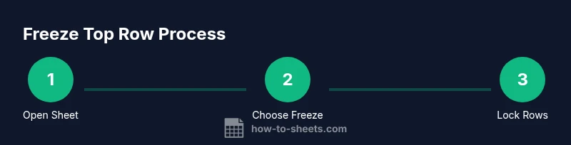
You can freeze the top row in Google Sheets to keep headers visible while scrolling. Open your sheet, go to View > Freeze, and select 1 row (or drag the thin gray line just below the header into position). This locks the header so it stays in place as you navigate data in the sheet.
Overview: why freezing the top row matters in Google Sheets\n\nFreezing the top row is a simple yet powerful habit for anyone working with datasets that have headers. When your data extends beyond the first screen, headers help you stay oriented and reduce misreading values. According to How To Sheets, adopting a consistent header-freezing approach improves data readability and reduces scrolling fatigue for students, professionals, and small business teams alike. The technique is universal across Google Sheets on desktop and mobile, which means you can lock headers once and reuse the same setup in different workbooks. In practical terms, this feature acts as a constant reference point for column labels like dates, names, IDs, and categories, so you never lose track while scanning rows of information.\n\nIn this guide we’ll cover not just the how, but the when and why, so you can decide the best freezing strategy for your specific workflow.
Quick methods to freeze the top row\n\nThere are multiple reliable ways to freeze the top row, depending on whether you prefer menus, drag handles, or keyboard shortcuts. The most common method is through the View menu: View > Freeze > 1 row. If you need more space for your headers, you can freeze two or more rows by selecting the row below the ones you want to lock, then applying Freeze again. Dragging the thin gray line above the top row is another intuitive approach—drag it down to lock 1 row or further to lock additional rows. This flexibility makes the top-row freeze practical for both simple and complex spreadsheets.\n\nFor users who share sheets, freezing options are preserved across viewers, ensuring everyone sees consistent headers as they scroll.
Keyboard shortcuts and quick actions\n\nKeyboard shortcuts can speed up the process when you’re working quickly. On Windows or Chrome OS, use the menu path: View > Freeze > 1 row. In some environments you can also access the freeze control via the right-click menu on the row header, depending on your browser and Google Sheets version. Mobile users can access a compact set of options within the app menu: tap the three-dot menu, choose Freeze, and select 1 row. These shortcuts and touch gestures keep headers visible without interrupting your workflow.
Common mistakes and how to avoid them\n\nA frequent error is freezing the wrong row, especially when headers are not the first row due to inserted rows or complex layouts. Always verify that row 1 contains your headers before freezing. If you accidentally freeze the wrong row, simply remove the freeze via View > Freeze > No rows, re-check the header row, and apply Freeze again. Also, avoid freezing different rows in different tabs of the same workbook unless you intend to standardize the header position across sheets.\n\nRemember that headers should be concise and consistently formatted to maximize readability when frozen.
Use cases across devices and Google Sheets versions\n\nFreezing headers works consistently on both desktop and mobile apps, although the exact menu wording can vary slightly between platforms. In desktop browsers, you’ll typically see View > Freeze. On mobile, look for the Freeze option within the app’s menu. If you collaborate across devices, the header lock persists when you open the sheet in other environments, provided you have edit permissions. This cross-platform stability makes the top-row freeze a dependable habit for teams that work in the cloud.
Troubleshooting: what to do if the top row won’t freeze\n\nIf freezing doesn’t work, first confirm you’re editing the correct sheet and that the top row truly contains header labels. Clear any filters or frozen panes in the current view that might conflict with the desired state. Try performing the operation in a new, blank sheet to ensure your Google Sheets settings aren’t interfering. If issues persist, refresh the page or sign out and back in to reset the session.\n\nIn most cases, reapplying View > Freeze > 1 row or dragging the divider resolves the problem quickly.
Advanced: freezing multiple rows or specific header behaviors\n\nSome datasets require locking more than one header row to maintain clarity. To freeze multiple rows, select the row beneath the last header you want to lock, then choose Freeze > 2 rows (or more), depending on your dataset structure. For datasets with multi-line headers, consider consolidating header text to fit a single line or reduce font size for readability when frozen. If you use filters, keep the freeze in mind, as filtered views can affect how headers align with data columns during heavy edits.
Best practices for headers and formatting\n\nKeep headers short and descriptive, using consistent capitalization and column order across sheets. When freezing, ensure the header row is not visually cluttered—thin borders, bold text, and clear alignment help a frozen header stay legible as you scroll. Pair freezing with conditional formatting or data validation for more robust sheet hygiene. Regularly review headers when you update data structures to avoid misalignment across frozen views.
Tools & Materials
- Computer or mobile device with internet(Google account access required to open Google Sheets)
- Target Google Sheets document(Ensure you have edit permissions)
- Optional: a test sheet or copy for experimentation(Safe space to practice freezing without affecting live data)
- External keyboard (optional)(Speeds up via keyboard shortcuts on desktop)
Steps
Estimated time: 5-10 minutes
- 1
Open the Google Sheet
Launch your Google Sheet in a browser or the mobile app and navigate to the sheet that contains headers you want to freeze.
Tip: If you’re collaborating, confirm you’re on the latest version by refreshing the page. - 2
Verify header row content
Ensure the first row contains your column headers and that there are no extra hidden rows above it that would misplace the header.
Tip: If headers are not in the first row, insert a new row above and move labels there before freezing. - 3
Apply the freeze via the menu
From the menu, select View > Freeze > 1 row to lock the top header row.
Tip: If you need more rows frozen, select below the header and choose 2 rows, 3 rows, etc. - 4
Confirm the header remains visible
Scroll down the sheet to verify the top header remains fixed in place across the viewport.
Tip: Try different zoom levels to ensure readability when frozen. - 5
Adjust if necessary
If the header shifts or disappears in some views, reapply the freeze and test on another tab or device.
Tip: Use the drag handle above the row header for a quick adjustment. - 6
Document the change
Note in your sheet's metadata or a project log that headers are frozen to prevent team confusion.
Tip: Include the date and user who performed the freeze.
FAQ
Can I freeze the top row on Google Sheets mobile app?
Yes. In the Google Sheets mobile app, open the sheet, tap the menu (three dots), choose Freeze, and select 1 row. The header will stay visible as you scroll.
Yes, you can freeze the top row on mobile by using Freeze in the app menu.
How do I unfreeze the top row?
Go to View > Freeze > No rows to remove the freezing. This returns the sheet to its default scrolling behavior.
To unfreeze, choose No rows in the Freeze menu.
Will freezing headers affect formulas or charts?
Freezing only affects the visible area and does not alter formulas or chart calculations. It simply keeps headers in view as you scroll.
Freezing headers doesn’t change formulas or charts; it just keeps the header visible.
Can I freeze headers in some sheets but not others in the same workbook?
Yes. Freezing is configured per sheet. You must apply the freeze on each sheet where you want headers to stay visible.
Freezing is per sheet, so apply it on each sheet as needed.
What if the header row is not the first row because of inserted data?
Move your header labels to the first row or insert a new row above and place headers there before freezing.
If headers aren’t in the first row, relocate them, then freeze.
Watch Video
The Essentials
- Freeze the header to maintain context while scrolling.
- Use View > Freeze to lock the top row and lock more rows if needed.
- Test freezing on multiple devices to ensure consistent behavior.
- Keep headers concise and consistently formatted for clarity.
- Document freezing actions to avoid confusion in collaborative work.