How to Freeze Panes in Google Sheets: Step-by-Step

Name: How to: Freeze Rows or Columns in Google Sheets
Uploaded: 2026-03-07
Duration: 18 s
Description: Master freezing panes in Google Sheets to keep headers visible while scrolling. This practical guide covers freezing top rows, left columns, and custom ranges, with tips for large datasets and working with filters.

Master freezing panes in Google Sheets to keep headers visible while scrolling. This practical guide covers freezing top rows, left columns, and custom ranges, with tips for large datasets and working with filters.

How To Sheets Team

March 7, 2026·5 min read

Google-Sheets-Free What-Is-Google-Sheets Open-In-Google-Sheets

Freeze Panes Guide - How To Sheets — Photo by 26797441via Pixabay

Quick AnswerSteps

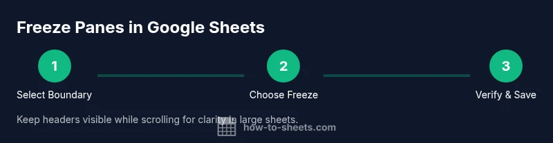
How to freeze panes in google sheets keeps headers visible as you scroll. In Google Sheets, freeze panes by selecting the boundary below the rows or to the right of the columns you want to lock, then choose View > Freeze. This method works for top rows, left columns, or a custom range across any sheet.

What freezing panes does in Google Sheets

Freezing panes locks selected rows and/or columns so they stay visible as you scroll through large spreadsheets. This keeps headers, labels, and reference data in view, reducing fatigue and helping you spot trends while comparing values across long datasets. If you’ve wondered how to freeze panes in google sheets, you’re in the right place. This technique applies consistently across sheets and devices, making data entry and review faster and more accurate. By freezing headers, you maintain context as you navigate rows, and by freezing columns you preserve column labels when scanning across dozens of fields. Across professional workflows—education, business, and analytics—freezing panes is a foundational skill that keeps critical information always in sight.

When to freeze panes: headers, labels, and sections

Knowing when to use freeze panes is about preserving context. Freeze the top header rows when your data has many rows; freeze the leftmost columns when you rely on row labels across many columns; and in complex workbooks, freeze a custom range to keep a specific header row and a key column visible at the same time. This ensures that when you scroll, you always know what each value represents. The approach also helps during data entry, auditing, and collaboration, where multiple users navigate the same sheet. By applying freezes thoughtfully, you reduce misreads and improve overall workflow efficiency.

Freezing options: top rows, left columns, and custom ranges

Google Sheets supports several freezing scenarios. You can freeze the top 1–10 rows to keep a multi-line header in view as your dataset grows. You can also freeze the leftmost 1–10 columns to anchor row labels. For more complex structures, you can freeze a custom range by selecting the cell at the intersection of the last row and last column you want frozen, then applying the freeze. This flexibility makes it easy to tailor freezes to the exact layout of your sheet, whether you’re building a budget, a schedule, or a student roster.

To apply freezes via the menu, open Google Sheets and select the boundary where you want the split. Go to the View menu, choose Freeze, and pick from options like 1 row, 2 rows, 1 column, 2 columns, or a custom range. This method is straightforward and reliable across browsers and devices. If you’re organizing a large dataset, freezing can prevent confusion by keeping headers and identifiers in view during scrolling. Remember to review your choices after applying them to ensure the correct rows and columns are locked.

Working with filters and large datasets: best practices

When your sheet includes filters or pivot-like views, freezing panes helps maintain context as you filter data or scroll through results. For large datasets, freeze just enough headers to preserve clarity without crowding the view. Consider freezing only the header row or the essential label column, then use other formatting features (like conditional formatting) to highlight important data. Regularly review frozen areas after adding new data to ensure the boundary still matches your intended layout. This practice makes ongoing data review smoother and less error-prone.

Troubleshooting common issues and mistakes

Common problems include freezing the wrong boundary or forgetting to update the freeze after inserting new rows or columns. If your headers disappear after scrolling, reapply the boundary by returning to View > Freeze and adjusting the selection. If you accidentally freeze too many rows or columns, simply choose No rows or No columns to unfreeze, then re-apply with the correct boundary. Always test a simple scroll after applying a freeze to confirm the pane stays in place. By avoiding over-freezing and keeping the boundary aligned with your data header, you’ll minimize layout surprises.

Best practices and gaps to watch for in real-world workbooks

In practical workbooks, plan freezes around the most-used headers and labels. For collaboration, document which panes are frozen so teammates understand the layout. When sharing, ensure your freeze choices remain sensible for viewers who may reopen the sheet on different screen sizes. Finally, pair freezing with clean dataset design—consistent header naming, stable column order, and thoughtful grouping—to maximize readability and efficiency across Google Sheets projects.

Tools & Materials

Device with internet access(Any computer, tablet, or phone with a modern browser)
Google account(Access to Google Sheets)
Open Google Sheets(Navigate via sheets.google.com)
Sample spreadsheet(Optional: practice before applying to workbooks)
Mouse or trackpad(Precise boundary selection helps)
Keyboard shortcuts reference(Useful for power users)

Steps

Estimated time: 5-10 minutes

1
Select the boundary where you want to freeze
Place the cursor on the row boundary below the headers you want frozen, or to the right of the column boundary you want locked. The exact boundary defines which rows and columns will stay in view when you scroll.
Tip: Hover near the divider to reveal the drag handle and ensure you pick the correct boundary.
2
Open the Freeze menu
Go to the top menu and choose View, then Freeze to access the available options. This reveals a quick set of choices you can apply with a single click.
Tip: If you don’t see the Freeze option, verify you selected a boundary in the sheet area (not in a chart or floating panel).
3
Choose the freeze option you need
Select from options like 1 row, 2 rows, 1 column, 2 columns, or a custom range. Your choice determines how many headers stay visible as you scroll.
Tip: For headers plus a key label column, pick a custom range that includes both the header row and the first column.
4
Verify the pane stays locked when scrolling
Scroll through the sheet to confirm the selected rows/columns remain visible. Adjust if needed by reopening the Freeze menu and changing the boundary.
Tip: If headers disappear during scrolling, reapply the boundary to ensure alignment.
5
Unfreeze when you’re ready
To remove a freeze, return to View > Freeze and choose No rows and No columns as applicable. This resets the pane behavior.
Tip: Unfreezing before restructuring data prevents misalignment later.
6
Document and share your layout
Note which rows and columns are frozen so collaborators understand the sheet structure. This reduces confusion when others edit or review the file.
Tip: Include a brief note in the sheet description or a dedicated 'Headers' tab to explain the freeze boundary.

Pro Tip: If your sheet has filters, consider freezing panes before applying filters to keep headers aligned.

Warning: Avoid freezing too many rows or columns; excessive freezes can clutter the view and slow navigation.

Note: You can freeze multiple rows and columns simultaneously by selecting the proper boundary (intersection cell) before applying Freeze.

FAQ

How do I freeze the top row in Google Sheets?

Place the cursor on the boundary under the top row and go to View > Freeze > 1 row. The top header will stay visible as you scroll down your data.

Can I freeze multiple rows or columns at once?

Yes. Select the cell at the intersection of the last row and last column you want frozen, then choose the appropriate Freeze option from the View menu. This locks both the chosen rows and columns simultaneously.

How do I unfreeze panes?

Open View > Freeze and select No rows and No columns to remove existing freezes. Your sheet will return to a fully scrollable view.

Does freezing panes affect printing a sheet?

Freezing panes affects on-screen navigation and print layouts. When printing, headers may repeat if you set print settings accordingly, but freezing itself is primarily an on-screen navigation aid.

Is there a keyboard shortcut to freeze panes?

There isn’t a single universal shortcut in Google Sheets for freezing panes; you typically use the View menu. Advanced users may script shortcuts via Google Apps Script for custom workflows.

What should I do if the Freeze option is missing?

Ensure you’ve clicked a cell within the worksheet area that defines a boundary. If necessary, refresh the page or reselect the boundary, then reopen View > Freeze.